Batch Multivalid Conformal Prediction

 

Our new paper gives very simple algorithms that promise "multivalid" conformal prediction sets for exchangable data. This means they are valid not just marginally, but also conditionally on (intersecting!) group membership, and in a threshold calibrated manner. I'll explain!

Instead of making point predictions, we can quantify uncertainty by producing "prediction sets" --- sets of labels that contain the true label with (say) 90% probability. The problem is, in a k label prediction problem, there are $2^k$ prediction sets. The curse of dimensionality!

One of the great ideas of conformal prediction is that if we can find a good "non-conformity score" s(x,y) telling us how unusual a label y seems for features x, we can focus on a 1-parameter family of prediction sets $P(x, t) = \{y : s(x,y) < t\}$. Now the problem is just to find $t$.

The usual recipe in split conformal prediction is to use a holdout set of points (x,y) to find a $t$ such that $\Pr[s(x,y) \leq t] = 0.9$. Then over the randomness of new examples (x,y), we have that $\Pr[y \in P(x,t)] = 0.9$. This is a -marginal- guarantee: the randomness is over x and y.

 

Suppose we have a bunch of groups (subsets of the feature space) g that we think are prediction-relevant? g could record e.g. demographic or other attributes of people. We might want to promise $\Pr[y \in P(x,t) | x \in g] = 0.9$. Vanilla split conformal doesn't promise this. 

 

If the groups g are disjoint, you could use a different threshold $t_g$ for each group --- but what if a single example can be a member of multiple groups? You can be conservative and use the largest threshold $t_g$ among all groups g that x is a member of, but this will over-cover.

 

The first insight here is that it no longer suffices to find a single threshold $t$ --- we need to find a function f mapping examples to thresholds, and to consider prediction sets $P(x,f(x)) =\{y : s(x,y) < f(x)\}$. The problem is to use a calibration set to train the function f. 

 

Our first algorithm is super simple and given any set of (intersecting!) groups G, trains f such that for every $g \in G$, we have that for new examples, $\Pr[y \in P(x,f(x))|g\in G] = 0.9$. How? f just minimizes pinball loss over linear combinations of group indicator functions $g \in G$. 

Now that we are using different thresholds f(x) for different x, you might worry that the threshold f(x) itself is correlated with coverage. To make sure its not, we can also ask for threshold calibration: $\Pr[y \in P(x,f(x)) | x \in g, f(x) = t] = 0.9$ for all $g \in G$ and all t. 

Our second algorithm trains f so that it has both group conditional and threshold calibrated coverage - what we call "full multivalid" coverage. It is also simple: It iteratively finds pairs $(g,t)$ on which multivalid coverage is violated empirically, and corrects the violations. 

 

This is the batch analogue of what we did in our NeurIPS 2022 paper in the sequential setting, which I wrote about here:  https://aaronsadventures.blogspot.com/2022/06/practical-robust-and-equitable.html The sequential setting is more difficult in many respects (no need to assume exchangable data!) but it requires labels at test time. Our new algorithms don't.

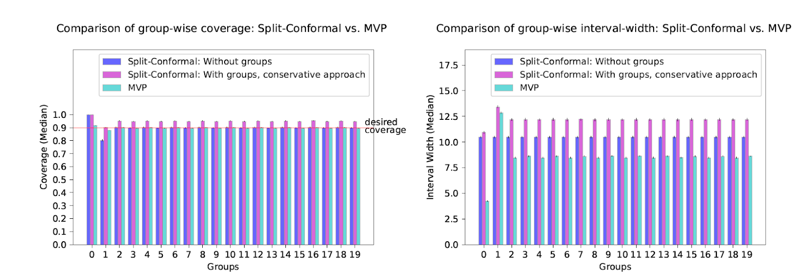
Both algorithms are very performant, taking a couple of seconds to train on thousands of points. Our first algorithm gets nearly perfect group conditional coverage on real datasets, and our second is never off by more than 1%, both improving significantly on baselines.

 

Our second algorithm gets better threshold calibration than our first (and compared to baselines), as expected. But perhaps surprisingly, our first algorithm performs quite well on calibration tests --- significantly beating baselines --- despite no formal calibration guarantees.

 

Our techniques come from the algorithmic fairness literature --- we train f to satisfy quantile analogues of multicalibration and multi-accuracy. If you haven't been paying attention to algorithmic fairness, maybe you should start --- there is interesting stuff going on there! Check out e.g. the Simons Collaboration on Algorithmic Fairness

This is joint work with the excellent Chris Jung, Georgy Noarov, and Ramya Ramalingam.

Our paper is here: https://arxiv.org/abs/2209.15145 and our code is here: https://github.com/ProgBelarus/BatchMultivalidConformal

 

Practical, Robust, and Equitable Uncertainty Estimation

This is a post about a new paper that is joint work with Bastani, Gupta, Jung, Noarov, and Ramalingam. The paper is here: https://arxiv.org/abs/2206.01067 and here is a recording of a recent talk I gave about it at the Simons Foundation: https://www.simonsfoundation.org/event/robust-and-equitable-uncertainty-estimation/ . This is cross-posted to the TOC4Fairness Blog (and this work comes out of the Simons Collaboration on the Theory of Algorithmic Fairness)

Machine Learning is really good at making point predictions --- but it sometimes makes mistakes. How should we think about which predictions we should trust? In other words, what is the right way to think about the uncertainty of particular predictions? Together with Osbert Bastani, Varun Gupta, Chris Jung, Georgy Noarov, and Ramya Ramalingam, we have some new work I'm really excited about. 

A natural way to quantify uncertainty is to predict a set of labels rather than a single one. Pick a degree of certainty --- say 90%. For every prediction we make, we'd like to return the smallest set of labels that is guaranteed to contain the true label 90% of the time. These are "prediction sets", and quantify uncertainty in a natural way: ideally, we will be sure about the correct label, and the prediction set will contain only a single label (the prediction we are certain about). But the larger our prediction set, the more our uncertainty, and the contents of the prediction set lets us know what exactly the model is uncertain about. 

An example of prediction sets for ImageNet. This example comes from a nice recent paper by Angelopoulos, Bates, Malik, and Jordan: https://arxiv.org/abs/2009.14193 

But how can we do this? Conformal Prediction provides a particularly simple way. Here is an outline of the vanilla version of conformal prediction (there are plenty of variants): 

Step 1: Pick a (non)conformity score to measure how different a label y is from a prediction f(x). e.g. for a regression model we could choose $s(x,y) = |f(x)-y|$ --- but lots of interesting work has been done recently to develop much fancier ones. A lot of the art of conformal prediction is in finding a good score function.

Step 2: Find a threshold $\tau$ such that for a new example $(x,y)$, $\Pr[s(x,y) \leq \tau] = 0.9$. An easy way to do this is using a holdout set. 

Step 3: On a new example $x$, given a point prediction $f(x)$, produce the prediction set $P(x) = \{y : s(x,y) \leq \tau\}$. 

Thats it! Nice and simple. Check out this recent survey by Angelopolous and Bates for an accessible introduction to conformal prediction. 

But a few things could go wrong. First, the technique of using a holdout set only works if the data is i.i.d. or more generally exchangable --- i.e. the data distribution should be permutation invariant. But maybe its coming from some changing distribution. If the distribution has changed in an expected and well behaved way, there are some fixes that let you apply the same framework, but if not you are likely in trouble.

A joke about non-exchangable data

Second, an average over everyone might not be what you care about. If we are in a personalized medicine setting, you might care about the reliability of predictions not just overall, but for women with a family history of diabetes and egg allergies --- or whatever else you think is medically relevant about you as an individual.

This is the problem that we want to solve: How to give prediction sets that cover their label 90% of the time even if we make no assumptions at all about the data generating process, and even if we care about coverage conditional on arbitrary intersecting subsets of the data.

We want stronger guarantees in another way too. If you think about our goal, there is a way to cheat: 90% of the time, predict the (trivial) set of all labels. 10% of the time predict the empty set. This covers the real label 90% of the time, but is completely uninformative.

To avoid this "solution", we also ask that our predictions be threshold calibrated. Remember our prediction sets have the form $P_t(x) = \{y : s(x,y) \leq \tau_t\}$. Now the threshold $\tau_t$ might be different every day. But we want 90% coverage even conditional on the value of $\tau_t$.

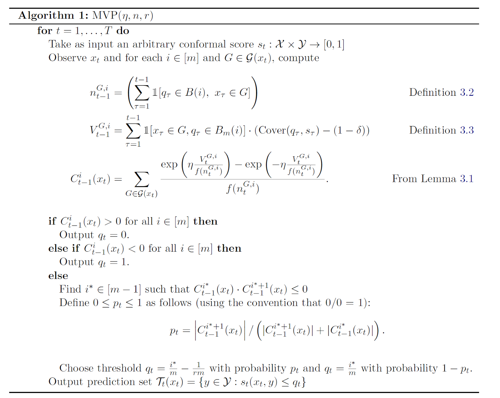
This rules out cheating. Remarkably (I think!), for every set of groups specified ahead of time, we're able to guarantee that even if the data is generated by an adversary, that our empirical coverage converges to 90% at the statistically optimal rate. Here is what that means:

Pick a threshold $\tau$ and group $G$. Consider all $n_{\tau,G}$ rounds in which the example $x$ was in $G$, and in which we predicted threshold $\tau$.  We promise that on this set, we cover 90% $\pm$ $1/\sqrt{n_{\tau,G}}$ of the labels. This is the best you could do even with a known distribution.

The best thing is that the algorithm is super simple and practical. We had a paper last year that showed how to do much of this in theory --- but the algorithm from that paper was not easily implementable (it involved solving an exponentially large linear program with a separation oracle).  But here is our new algorithm --- it only involves doing a small amount of arithmetic for each prediction:

So we're able to implement it and run a bunch of experiments. You can read about them in detail in the paper, but the upshot is that our new method is competitive with split conformal prediction even on "its own turf" --- i.e. when the data really is drawn i.i.d. and we only care about marginal coverage --- and really excels when the data comes from a more complicated source, or when we measure group-conditional coverage, which traditional methods tend to have much more trouble with. We run experiments on regression and classification tasks, on exchangeable data, under distribution shift, on real time series data, and on adversarial data orderings. Even when the data is i.i.d. and we only care about marginal coverage, our method has an important advantage over split conformal prediction --- since we don't need to preserve exchangability, we can use all of the data to train the underlying model, whereas split conformal prediction needs to reserve some fraction of it for a holdout set. The result is faster learning for our method, which results in smaller/more accurate prediction sets even without the complicating factors of groupwise coverage, threshold calibration or adversarial data!