Practical, Robust, and Equitable Uncertainty Estimation

This is a post about a new paper that is joint work with Bastani, Gupta, Jung, Noarov, and Ramalingam. The paper is here: https://arxiv.org/abs/2206.01067 and here is a recording of a recent talk I gave about it at the Simons Foundation: https://www.simonsfoundation.org/event/robust-and-equitable-uncertainty-estimation/ . This is cross-posted to the TOC4Fairness Blog (and this work comes out of the Simons Collaboration on the Theory of Algorithmic Fairness)

Machine Learning is really good at making point predictions --- but it sometimes makes mistakes. How should we think about which predictions we should trust? In other words, what is the right way to think about the uncertainty of particular predictions? Together with Osbert Bastani, Varun Gupta, Chris Jung, Georgy Noarov, and Ramya Ramalingam, we have some new work I'm really excited about. 

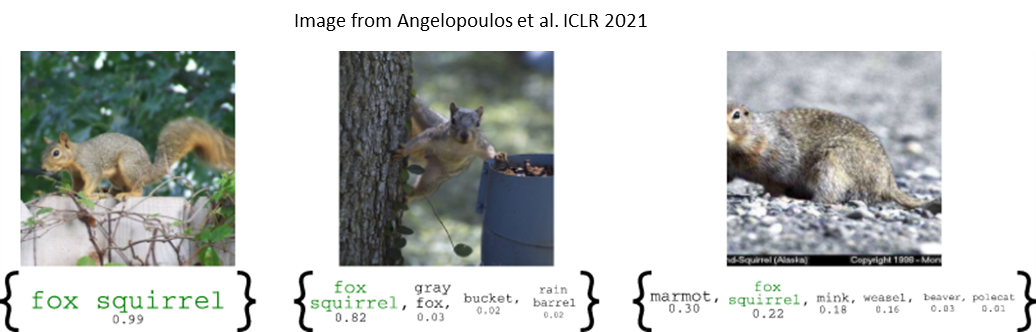
A natural way to quantify uncertainty is to predict a set of labels rather than a single one. Pick a degree of certainty --- say 90%. For every prediction we make, we'd like to return the smallest set of labels that is guaranteed to contain the true label 90% of the time. These are "prediction sets", and quantify uncertainty in a natural way: ideally, we will be sure about the correct label, and the prediction set will contain only a single label (the prediction we are certain about). But the larger our prediction set, the more our uncertainty, and the contents of the prediction set lets us know what exactly the model is uncertain about. 

An example of prediction sets for ImageNet. This example comes from a nice recent paper by Angelopoulos, Bates, Malik, and Jordan: https://arxiv.org/abs/2009.14193 

But how can we do this? Conformal Prediction provides a particularly simple way. Here is an outline of the vanilla version of conformal prediction (there are plenty of variants): 

Step 1: Pick a (non)conformity score to measure how different a label y is from a prediction f(x). e.g. for a regression model we could choose $s(x,y) = |f(x)-y|$ --- but lots of interesting work has been done recently to develop much fancier ones. A lot of the art of conformal prediction is in finding a good score function.

Step 2: Find a threshold $\tau$ such that for a new example $(x,y)$, $\Pr[s(x,y) \leq \tau] = 0.9$. An easy way to do this is using a holdout set. 

Step 3: On a new example $x$, given a point prediction $f(x)$, produce the prediction set $P(x) = \{y : s(x,y) \leq \tau\}$. 

Thats it! Nice and simple. Check out this recent survey by Angelopolous and Bates for an accessible introduction to conformal prediction. 

But a few things could go wrong. First, the technique of using a holdout set only works if the data is i.i.d. or more generally exchangable --- i.e. the data distribution should be permutation invariant. But maybe its coming from some changing distribution. If the distribution has changed in an expected and well behaved way, there are some fixes that let you apply the same framework, but if not you are likely in trouble.

A joke about non-exchangable data

Second, an average over everyone might not be what you care about. If we are in a personalized medicine setting, you might care about the reliability of predictions not just overall, but for women with a family history of diabetes and egg allergies --- or whatever else you think is medically relevant about you as an individual.

This is the problem that we want to solve: How to give prediction sets that cover their label 90% of the time even if we make no assumptions at all about the data generating process, and even if we care about coverage conditional on arbitrary intersecting subsets of the data.

We want stronger guarantees in another way too. If you think about our goal, there is a way to cheat: 90% of the time, predict the (trivial) set of all labels. 10% of the time predict the empty set. This covers the real label 90% of the time, but is completely uninformative.

To avoid this "solution", we also ask that our predictions be threshold calibrated. Remember our prediction sets have the form $P_t(x) = \{y : s(x,y) \leq \tau_t\}$. Now the threshold $\tau_t$ might be different every day. But we want 90% coverage even conditional on the value of $\tau_t$.

This rules out cheating. Remarkably (I think!), for every set of groups specified ahead of time, we're able to guarantee that even if the data is generated by an adversary, that our empirical coverage converges to 90% at the statistically optimal rate. Here is what that means:

Pick a threshold $\tau$ and group $G$. Consider all $n_{\tau,G}$ rounds in which the example $x$ was in $G$, and in which we predicted threshold $\tau$.  We promise that on this set, we cover 90% $\pm$ $1/\sqrt{n_{\tau,G}}$ of the labels. This is the best you could do even with a known distribution.

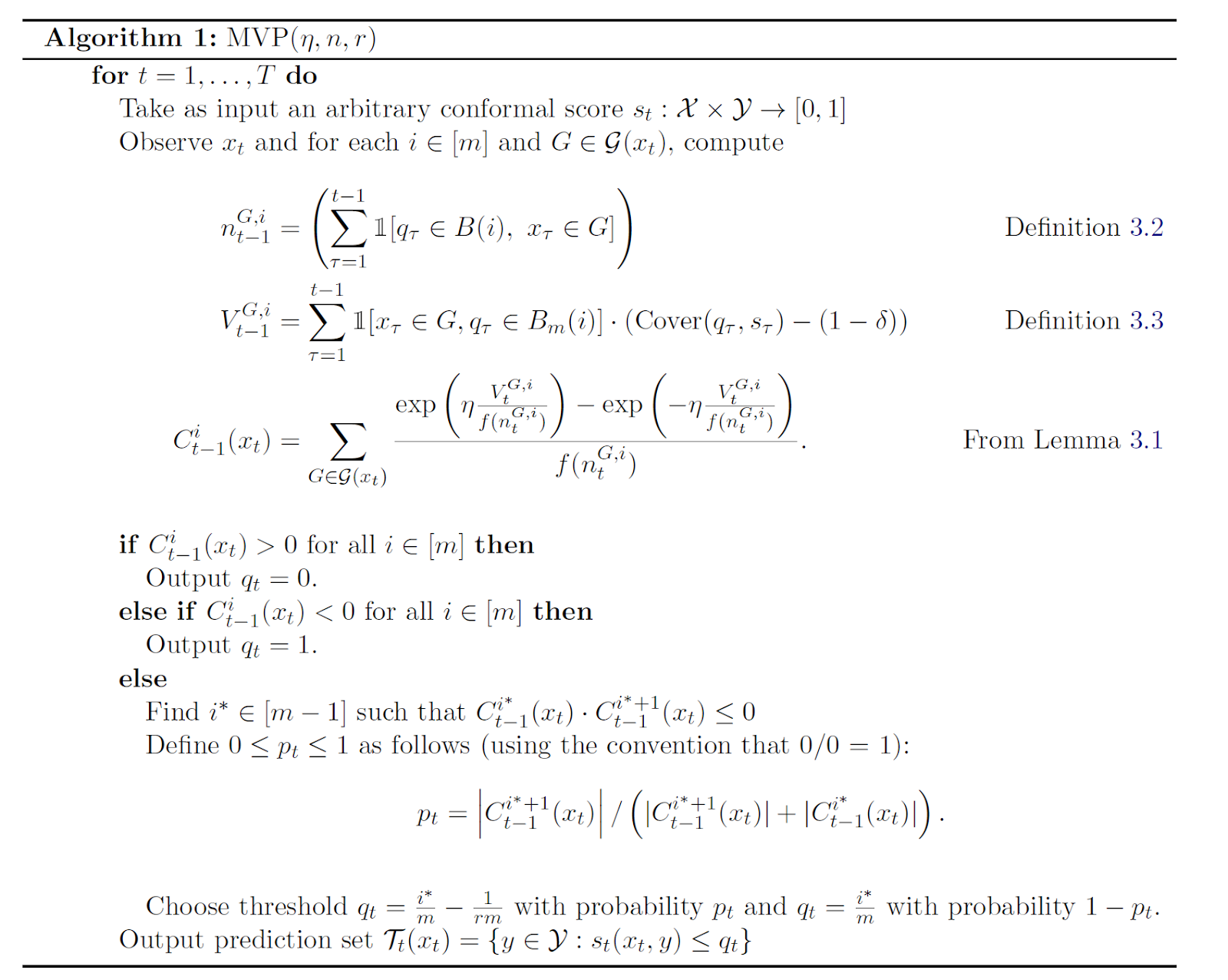
The best thing is that the algorithm is super simple and practical. We had a paper last year that showed how to do much of this in theory --- but the algorithm from that paper was not easily implementable (it involved solving an exponentially large linear program with a separation oracle).  But here is our new algorithm --- it only involves doing a small amount of arithmetic for each prediction:

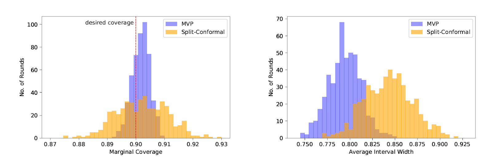
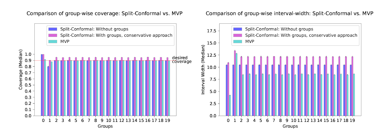
So we're able to implement it and run a bunch of experiments. You can read about them in detail in the paper, but the upshot is that our new method is competitive with split conformal prediction even on "its own turf" --- i.e. when the data really is drawn i.i.d. and we only care about marginal coverage --- and really excels when the data comes from a more complicated source, or when we measure group-conditional coverage, which traditional methods tend to have much more trouble with. We run experiments on regression and classification tasks, on exchangeable data, under distribution shift, on real time series data, and on adversarial data orderings. Even when the data is i.i.d. and we only care about marginal coverage, our method has an important advantage over split conformal prediction --- since we don't need to preserve exchangability, we can use all of the data to train the underlying model, whereas split conformal prediction needs to reserve some fraction of it for a holdout set. The result is faster learning for our method, which results in smaller/more accurate prediction sets even without the complicating factors of groupwise coverage, threshold calibration or adversarial data!

FORC 2021 Call for Papers

 Reminder to anyone who has forgotten about FORC 2021 --- its a very nice venue --- and also a nice place to highlight recent work that is published or submitted elsewhere, via the non-archival track.

Symposium on Foundations of Responsible Computing (FORC) 2021 Call for Papers - Deadline February 15, 2021 AOE (anywhere on Earth)

The second annual Symposium on Foundations of Responsible Computing (FORC) is planned to be held on June 9-11, 2021, *online*. FORC is a forum for mathematically rigorous research in computation and society writ large.  The Symposium aims to catalyze the formation of a community supportive of the application of theoretical computer science, statistics, economics, and other relevant analytical fields to problems of pressing and anticipated societal concern.

Topics that fall in scope include, but are not restricted to, formal approaches to privacy, including differential privacy; theoretical approaches to fairness in machine learning, including the investigation of definitions, algorithms and lower bounds, tradeoffs, and economic incentives; computational and mathematical social choice (including apportionment and redistricting); theoretical foundations of sustainability; mechanism design for social good; mathematical approaches to bridging computer science, law and ethics; and theory related to modeling and mitigating the spread of epidemics. The Program Committee also warmly welcomes mathematically rigorous work on societal problems that have not traditionally received attention in the theoretical computer science literature. Whatever the topic, submitted papers should communicate their contributions towards responsible computing, broadly construed.

The symposium itself will feature a mixture of talks by authors of accepted papers and invited talks. At least one author of each accepted paper should be present at the symposium to present the work (with an option for virtual attendance, as needed).

Dual Submission Policy. Authors must indicate at the time of submission whether they are submitting to the archival-option track or the non-archival track.

* For submissions to the non-archival track, it is permitted to submit papers that have appeared in a peer-reviewed conference or journal since the last FORC. It is also permitted to simultaneously or subsequently submit substantially similar work to another conference or to a journal. Accepted papers in the non-archival track will receive talks at the symposium and will appear as one-page abstracts on the symposium website. They will not appear in the proceedings.

* For submissions to the archival-option track, papers that are substantially similar to papers that have been previously published, accepted for publication, or submitted in parallel to other peer-reviewed conferences with proceedings may not be submitted. Also, submissions that are substantially similar to papers that are already published in a journal at the time of submission may not be submitted to the archival-option track. Accepted papers in the archival-option track will receive talks at the symposium. Authors of papers accepted to the archival-option track will be given the option to choose whether to convert to a one-page abstract (which will not appear in the proceedings) or publish a 10-page version of their paper in the proceedings. The proceedings of FORC 2021 will be published by LIPIcs.

Authors are also responsible for ensuring that submitting to FORC would not be in violation of other journals’ or conferences’ submission policies.

PC members and reviewers will be aware during the review process of whether papers have been submitted as archival-option or non-archival. The PC reserves the right to hold non-archival papers to a different standard than archival-option papers.

Submission Instructions.
* Authors should upload a PDF of the paper here: https://easychair.org/conferences/?conf=forc2021.
* A footnote on the title of the paper should indicate whether the paper is a submission to the archival-option track or the non-archival track. Submissions to the non-archival track should also indicate in this footnote any archival venues (conferences or journals) at which the paper has appeared, a link to the publication, and the date on which it was published.
* The font size should be at least 11 point and the format should be single-column.
* Author names and affiliations should appear at the top of the paper (reviewing for FORC is single, not double blind).
* Beyond these, there are no formatting or length requirements, but reviewers will only be asked to read the first 10 pages of the submission. It is the authors’ responsibility that the main results of the paper and their significance be clearly stated within the first 10 pages. For both the archival-option track and the non-archival track, submissions should include proofs of all central claims, and the committee will put a premium on writing that conveys clearly and in the simplest possible way what the paper is accomplishing.
* Authors are free to post their submissions on arXiv or other online repositories.


All questions about submissions should be emailed to the PC chair, Katrina Ligett, at katrina@cs.huji.ac.il

FORC Steering Committee

Avrim Blum
Cynthia Dwork      
Shafi Goldwasser  
Sampath Kannan
Jon Kleinberg
Kobbi Nissim  
Toni Pitassi
Omer Reingold
Guy Rothblum  
Salvatore Ruggieri
Salil Vadhan
Adrian Weller


FORC 2021 Program Committee

Borja Balle
Raef Bassily
Mark Bun
Elisa Celis
Aloni Cohen
Moon Duchin
Vitaly Feldman
Kira Goldner
Krishna Gummadi
Swati Gupta
Gautam Kamath
Michael Kearns
Scott Kominers
Himabindu Lakkaraju
Katrina Ligett (chair)
Jamie Morgenstern
Seth Neel
Kobbi Nissim
Adam Smith
Kunal Talwar
Salil Vadhan

Important Dates

Submission deadline: February 15, 2021 AOE (anywhere on Earth)
Author notification: March 31, 2021
Conference: June 9-11, 2021

How to Estimate the Uncertainty of Predictions

This is a post about a new paper Online Multivalid Learning: Means, Moments, and Prediction Intervals, that is joint work with Varun Gupta, Christopher Jung, Georgy Noarov, and Mallesh Pai. It is cross-posted to the new TOC4Fairness blog. For those that prefer watching to reading, here is a recording of a talk I gave on this paper. 

Suppose you go and train the latest, greatest machine learning architecture to predict something important. Say (to pick an example entirely out of thin air) you are in the midst of a pandemic, and want to predict the severity of patients' symptoms in 2 days time, so as to triage scarce medical resources. Since you will be using these predictions to make decisions, you would like them to be accurate in various ways: for example, at the very least, you will want your predictions to be calibrated, and you may also want to be able to accurately quantify the uncertainty of your predictions (say with 95% prediction intervals). It is a fast moving situation, and data is coming in dynamically --- and you need to make decisions as you go. What can you do?

The first thing you might do is ask on twitter! What you will find is that the standard tool for quantifying uncertainty in settings like this is conformal prediction. The conformal prediction literature has a number of elegant techniques for endowing arbitrary point prediction methods with marginal prediction intervals: i.e intervals $(\ell(x), u(x))$ such that over the randomness of some data distribution over labelled examples $(x,y)$: $\Pr_{(x,y)}\left[y \in [\ell(x), u(x)]\right] \approx 0.95$ These would be 95% marginal prediction intervals --- but in general you could pick your favorite coverage probability $1-\delta$.

Conformal prediction has a lot going for it --- its tools are very general and flexible, and lead to practical algorithms. But it also has two well known shortcomings:

1. Strong Assumptions. Like many tools from statistics and machine learning, conformal prediction methods require that the future look like the past. In particular, they require that the data be drawn i.i.d. from some distribution --- or at least be exchangable (i.e. their distribution should be invariant to permutation). This is sometimes the case --- but it often is not. In our pandemic scenario, the distribution on patient features might quickly change in unexpected ways as the disease moves between different populations, as might the relationship between features and outcomes, as treatments advance. In other settings in which consequential decisions are being made about people --- like lending and hiring decisions --- people might intentionally manipulate their features in response to the predictive algorithms you deploy, in an attempt to get the outcome they want. Or you might be trying to predict outcomes in time series data, in which there are explicit dependencies across time. In all of these scenarios, exchangeability is violated.
2. Weak Guarantees. Marginal coverage guarantees are averages over people. 95% marginal coverage means that the true label falls within the predicted interval for 95% of people. It need not mean anything for people like you. For example, if you are part of a demographic group that makes up less than 5% of the population, it is entirely consistent with the guarantees of a 95% marginal prediction interval that labels for people from your demographic group fall outside of their intervals 100% of the time. This can be both an accuracy and a fairness concern --- marginal prediction works well for "typical" members of a population, but not necessarily for everyone else.

What kinds of improvements might we hope for? Lets start with how to strengthen the guarantee:

Multivalidity Ideally, we would want conditional guarantees --- i.e. the promise that for every $x$, that we would have $\Pr_{y}\left[y \in [\ell(x), u(x)] | x \right] \approx 0.95$. In other words, that somehow for each individual, the prediction interval was valid for them specifically, over the "unrealized" (or unmeasured) randomness of the world. Of course this is too much to hope for. In a rich feature space, we have likely never seen anyone exactly like you before (i.e. with your feature vector $x$). So strictly speaking, we have no information at all about your conditional label distribution. We still have to average over people. But we don't have to average over everybody. An important idea that has been investigated in several different contexts in recent years in the theory literature on fairness is that we might articulate a very rich collection of (generally intersecting) demographic groups $G$ corresponding to relevant subsets of the data domain, and ask for things that we care about to hold true as averaged over any group $S \in G$ in the collection. In the case of prediction intervals, this would correspond to asking for something like that simultaneously for every demographic group $S \in G$, $\Pr_{(x,y)}\left[y \in [\ell(x), u(x)] | x \in S \right] \approx 0.95$. Note here that an individual might be a member of many different demographic groups, and can interpret the guarantees of their prediction interval as averages over any of those demographic groups, at their option. This is what we can achieve --- at least for any such group that isn't too small. 

And what kinds of assumptions do we need?

Adversarial Data Actually, its not clear that we need any! Many learning problems which initially appear to require distributional assumptions turn out to be solvable even in the worst case over data sequences --- i.e. even if a clever adversary, with full knowledge of your algorithm, and with the intent only to sabotage your learning guarantees, is allowed to adaptively choose data to present to your algorithm. This is the case for calibrated weather prediction, as well as general contextual prediction. It turns out to be the case for us as well. Instead of promising coverage probabilities of $1-\delta + O(1/T)$ after $T$ rounds on the underlying distribution, as conformal prediction is able to, (for us there is no underlying distribution) we offer empirical coverage rates of $1-\delta \pm O(1/\sqrt{T})$. This kind of guarantee is quite similar to what conformal prediction guarantees about empirical coverage.

More Generally Our techniques are not specific to prediction intervals. We can do the same thing for predicting label means, and predicting variances of the residuals of arbitrary prediction methods. For mean prediction, this corresponds to an algorithm for providing multi-calibrated predictions in the sense of Hebert-Johnson et al, in an online adversarial environment. For variances and other higher moments, it corresponds to an online algorithm for making mean-conditioned moment multicalibrated predictions in the sense of Jung et al.

Techniques At the risk of boring my one stubbornly remaining reader, let me say a few words about how we do it. We generalize an idea that dates back to an argument that Fudenberg and Levine first made in 1995 --- and is closely related to an earlier, beautiful argument by Sergiu Hart --- but that I just learned about this summer, and thought was just amazing. It applies broadly to solving any prediction task that would be easy, if only you were facing a known data distribution. This is the case for us. If, for each arriving patient at our hospital, a wizard told us their "true" distribution over outcome severity, we could easily make calibrated predictions by always predicting the mean of this distribution --- and we could similarly read off correct 95% coverage intervals from the CDF of the distribution. So what? That's not the situation we are in, of course. Absent a wizard, we first need to commit to some learning algorithm, and only then will the adversary decide what data to show us.

But lets put our game theory hats on. Suppose we've been making predictions for awhile. We can write down some measure of our error so far --- say the maximum, over all demographic groups in $G$, of the deviation of our empirical coverage so far from our 95% coverage target. For the next round, define a zero sum game, in which we (the learner) want to minimize the increase in this measure of error, and the adversary wants to maximize it. The defining feature of zero-sum games is that how well you can do in them is independent of which player has to announce their distribution on play first --- this is the celebrated Minimax Theorem. So to evaluate how well the learner could do in this game, we can think about the situation involving a Wizard above, in which for each arriving person, before we have to make a prediction for them, we get to observe their true label distribution. Of course in this scenario we can do well, because for all of our goals, our measure of success is based on how well our predictions match observed properties of these distributions. The Minimax theorem tells us that (at least in principle --- it doesn't give us the algorithm), there must therefore also be a learning algorithm that can do just as well, but against an adversary.

The minimax argument is slick, but non-constructive. To actually pin down a concrete algorithm, we need to solve for the equilibrium in the corresponding game. That's what we spend much of the paper doing, for each of the prediction tasks that we study. For multicalibration, we get a simple, elementary algorithm --- but for the prediction interval problem, although we get a polynomial time algorithm, it involves solving a linear program with a separation oracle at each round. Finding more efficient and practical ways to do this strikes me as an important problem.

Finally, I had more fun writing this paper --- learning about old techniques from the game theoretic calibration literature --- than I've had in awhile. I hope a few people enjoy reading it!

 

No Regret Algorithms from the Min Max Theorem

The existence of no-regret learning algorithms can be used to prove Von-Neumann's min-max theorem. This argument is originally due to Freund and Schapire, and I teach it to my undergraduates in my algorithmic game theory class. The min-max theorem also can be used to prove the existence of no-regret learning algorithms. Here is a constructive version of the argument (Constructive in that in the resulting algorithm, you only need to solve polynomially sized zero-sum games, so you can do it via linear programming).

Recall the setting. Play proceeds in rounds $t \in \{1,\ldots,T\}$. At each day $t$, the learner chooses one of $k$ actions $i_t \in \{1,\ldots,k\}$, and the adversary chooses a loss vector $\ell^t \in [0,1]^k$. The learner incurs loss $\ell^t_{i_t}$, corresponding to the action he chose. At the end of the interaction, the regret of the learner is defined to be the difference between the cumulative loss he incurred and the cumulative loss of the best fixed action (played consistently)  in hindsight:

$$\textrm{Regret}_T = \max_j \left(\sum_{t=1}^T \ell^t_{i_t} - \ell^t_j\right)$$ 

A classical and remarkable result is that there exist algorithms that can guarantee that regret grows only sublinearly with time: $\textrm{Regret}_T = O(\sqrt{T})$. Lets prove this. 

Define the non-negative portion of our cumulative regret with respect to action $j$ up until day $d$ as:

$$V_d^j = \left(\sum_{t=1}^d\left(\ell^t_{i_t} - \ell^t_j\right)\right)^+$$

and our additional regret at day $d+1$ with respect to action $j$ as:

$$r_{j}^{d+1} = \ell_{i_{d+1}}^{d+1} - \ell^{d+1}_j$$

Observe that if $V_{d}^j \geq 1$  then $V_{d+1}^j = V_d^j + r_j^{d+1}$. 

Define a surrogate loss function as our squared cumulative regrets, summed over all actions: 

$$L_d = \sum_{j=1}^k (V_d^j)^2$$

Observe that we can write the expected gain in our loss on day $d+1$, conditioned on the history thus far:

$$\mathbb{E}[L_{d+1} - L_d] \leq \sum_{j : V_d^j \geq 1} \mathbb{E}[(V_d^j+r_j^{d+1})^2 - (V_d^j)^2) ] + 3k$$

$$= \sum_{j : V_d^j \geq 1} \left(2V_d^j \mathbb{E}[r_{j}^{d+1}] + \mathbb{E}[(r_{j}^{d+1})^2]\right) + 3k $$

$$\leq \sum_{j=1}^k \left(2V_d^j \mathbb{E}[r_{j}^{d+1}]\right) + 4k$$

where the expectations are taken over the randomness of both the learner and the adversary in round $d+1$. 

Now consider a zero-sum game played between the learner and the adversary in which the learner is the minimization player, the adversary is the maximization player, and the utility function is $$u(i_{d+1}, \ell^{d+1}) = \sum_{j=1}^k \left(2V_d^j \mathbb{E}[r_{j}^{d+1}]\right)$$ The min-max theorem says that the learner can guarantee the same payoff for herself in the following two scenarios:

1. The learner first has to commit to playing a distribution $p_{d+1}$ over actions $i$, and then the adversary gets to best respond by picking the worst possible loss vectors, or
2. The adversary has to first commit to a distribution over loss vectors $\ell$ and then the learner gets the benefit of picking the best action $i_{d+1}$ to respond with. 

Scenario 1) is the scenario our learner finds herself in, when playing against an adaptive adversary. But 2) is much easier to analyze. If the adversary first commits to a distribution over loss vectors $\ell^{d+1}$, the learner can always choose action $i_{d+1} = \arg\min_j \mathbb{E}[\ell^{d+1}_j]$, which guarantees that $\mathbb{E}[r_{j}^{d+1}] \leq 0$, which in turn guarantees that the value of the game $ \sum_{j=1}^k \left(2V_d^j \mathbb{E}[r_{j}^{d+1}]\right) \leq 0$.  Hence, the min-max theorem tells us that the learner always has a distribution over actions $p_{d+1}$ that guarantees that $\mathbb{E}[L_{d+1} - L_d] \leq 4k$, even in the worst case over loss functions. If the learner always plays according to this distribution, then by a telescoping sum, we have that:

$$\mathbb{E}[L_T] \leq 4kT$$.

We therefore have by Jensen's inequality that:

$$\mathbb{E}[\max_j (V^j_T)] \leq \sqrt{\mathbb{E}[\max_j (V^j_T)^2]}\leq \sqrt{\mathbb{E}[\sum_{j=1}^k (V_j^T)^2]} \leq 2\sqrt{kT}$$.

Moment Multicalibration for Uncertainty Estimation

This blog post is about a new paper that I'm excited about, which is joint work with Chris Jung, Changhwa Lee, Mallesh Pai, and Ricky Vohra. If you prefer watching talks, you can watch one I gave to the Wharton statistics department here.

Suppose you are diagnosed with hypertension, and your doctor recommends that you take a certain drug to lower your blood pressure. The latest research, she tells you, finds that the drug lowers diastolic blood pressure by an average of 10 mm Hg. You remember your statistics class from college, and so you ask about confidence intervals. She looks up the paper, and tells you that it reports a 95% confidence interval of [5, 15]. How should you interpret this? 

What you might naively hope is that [5, 15] represents a conditional prediction interval. If you have some set of observable features $x$, and a label $y$ (in this case corresponding to your decrease in diastolic blood pressure after taking the drug), a 95% conditional prediction interval would promise that:

$$\Pr_y [y \in [5, 15] | x] \geq 0.95$$

In other words, a conditional prediction interval would promise that given all of your observed features, over the unrealized/unmeasured randomness of the world, there is a 95% chance that your diastolic blood pressure will decrease by between 5 and 15 points. 

But if you think about it, coming up with a conditional prediction interval is essentially impossible in a rich feature space. If $x$ contains lots of information about you, then probably there was nobody in the original study population that exactly matched your set of features $x$, and so we have no information at all about the conditional distribution on $y$ given $x$ --- i.e. no samples at all from the distribution over which our coverage probability supposedly holds! So how can you expect any sort of promise at all? There are two typical ways around this difficulty. 

The first is to make heroic assumptions about the data generation process. For example, if we assume that the world looks like an ordinary least squares model, and that there is a linear relationship between $y$ and $x$, then we can form a confidence region around the parameters of the model, and from that derive prediction intervals. But these prediction intervals are not valid if the model fails to hold, which it inevitably will. 

The second is to give up on conditional prediction intervals, and instead give marginal prediction intervals. This is what the conformal prediction literature aims to do. A marginal prediction interval looks quite similar to a conditional prediction interval (at least syntactically), and promises:

$$\Pr_{(x,y)} [y \in [5, 15] ] \geq 0.95$$

Rather than conditioning on your features $x$, a marginal prediction interval averages over all people, and promises that 95% of people who take the drug have their diastolic blood pressure lowered by between 5 and 15 points. But the semantics of this promise are quite different than that of a conditional prediction interval. Because the average is now taken over a large, heterogeneous population, very little is promised to you. For example, it might be that for patients in your demographic group (e.g. middle aged women with Sephardic Jewish ancestry and a family history of diabetes) that the drug is actually expected to raise blood pressure rather than lower it. Because this subgroup represents less than 5% of the population, it is entirely consistent with the marginal prediction interval being correct. Of course, if you are lucky, then perhaps someone has conducted a study of people from this demographic group and has computed marginal prediction intervals over it! But what if there are multiple different groups that you are a member of, over which the results seem to conflict? For example, you might also have a low BMI value and have unusually good cholesterol readings --- features of a group for which the drug works unusually well. Which uncertainty estimate should you trust, if you are a member of both groups? 

These concerns actually arise already when we think about the semantics of mean estimations ("the expected drop in blood pressure amongst patients who take this drug is 10 mm Hg"). Ideally, if you were a patient with features $x$, then 10 would be an estimate of $\mathbb{E}[y | x]$. But just as with uncertainty estimation, in a large feature space, we typically have no information about the distribution on $y$ conditional on $x$ (because we have never met anyone exactly like you before), and so instead what we have is just an estimate of $\mathbb{E}[y]$ --- i.e. averaging over people. If you have a method of making predictions $f(x)$ as a function of features $x$, then a standard performance metric is calibration --- which informally asks that for every prediction $p$, amongst all people for whom we predicted $f(x) = p$, the average of the realized labels $y$ should be $p$. Again, estimates of this form promise little to individuals, because they are averages over a large and heterogeneous population.   

Several years ago, Hebert-Johnson et al. proposed a nice way to interpolate between the (impossible) ideal of offering conditional mean predictions  $f(x) = \mathbb{E}[y | x]$, and the weak guarantee of merely offering calibrated predictions $f$. Roughly speaking, they proposed to specify a very large collection of potentially intersecting groups $G$ (representing e.g. demographic groups like Sephardic Jewish women with a family history of diabetes, and hypertensive patients with low cholesterol and BMI values, etc) and to ask that a trained predictor be simultaniously calibrated on each sufficiently large group in $G$. They showed how to accomplish this using a polynomially sized sample from the underlying distribution, with polynomial running time overhead, on top of the cost of solving learning problems over $G$. 

In our paper, we --- roughly speaking --- show how to accomplish the same thing, but for variances and other higher moments, in addition to just means. And our "multicalibrated moment estimates" can be used to construct prediction intervals in exactly the same way that real moments of the conditional label distribution could be used. If you used the real (unknown) label distribution moments, you would have gotten conditional prediction intervals. If you use our multi-calibrated moments, you get marginal prediction intervals that are simultaneously valid as averaged over each of the groups in $G$. So, for example, our hypertensive patient above could interpret her prediction interval --- if it was constructed from multicalibrated moment estimates computed from her features --- as an average over each of the demographic groups that she is a member of (so long as they are contained within $G$), and all of those interpretations would be simultaneously valid. 

I'll leave the details to the paper --- including what exactly we mean by "moment multicalibration". I'll just note that a major difficulty is that variances and higher moments --- unlike expectations --- do not combine linearly, so it is no longer sensible to ask that "amongst all people for whom we predicted variance v, the true variance should be v" --- because even the true conditional label variances do not satisfy this property. But it is sensible to ask that a pair of mean and moment predictions be calibrated in this way: "amongst all people for whom we predicted mean $\mu$ and variance v, the true mean should be $\mu$ and the true variance should be $v$." This is what we call "mean-conditioned moment calibration", and it is satisfied by the true distributional moments. 

The paper is here: Moment Multicalibration for Uncertainty Estimation.

TCS Visioning Workshop — Call for Participation

Reposting from here: https://thmatters.wordpress.com/2020/06/05/tcs-visioning-workshop-call-for-participation/

The CATCS will be hosting a virtual “Visioning Workshop” the week of July 20 in order to identify broad research themes within theoretical computer science (TCS) that have potential for a major impact in the future. The goals are similar to the workshop of the same name in 2008: to package these themes in a way that can be consumed by the general public, which we would deliver primarily to the Computing Community Consortium and others (e.g. funding agencies) to help them advocate for TCS.

While participation in the workshop is primarily through invitation, we have a few slots available for the broader community. If you are interested in participating, please see details of the application process below. The workshop will be organized according to area-wise breakout groups. Each breakout group will have 1-2 leads. Breakout groups will meet for 4-5 hours spread across several days and will be tasked with brainstorming ideas and preparing materials related to their topic. Leads are further expected to participate in plenary sessions held on Monday July 20 and Friday July 24 (4-5 hrs of additional time) where these materials will be discussed.

If you are interested in participating in the workshop, please fill out this Google form by Monday June 15. On this form, applicants are asked to contribute one or two major results in the last 10 years whose significance can be explained in layperson terms, and one or two major challenges for theory whose significance can be explained in layperson terms. These descriptions can be very brief. We will just use them to select participants and create breakout groups.

FORC 2020 Program

The FORC 2020 program is now available here: https://responsiblecomputing.org/program/ (and reproduced below) Note the terrific set of contributed talks at keynotes, and note that registration is free! There will also be junior/senior breakout sessions into small groups during the lunch breaks to facilitate informal conversation and networking. Please consider attending, and help to spread the word!

FORC 2020 will take place virtually (on Zoom) on June 1st and 2nd, 2020. All times below are in Eastern Daylight Time (i.e. Boston/New York/Philadelphia time).

Registration is FREE but mandatory (Zoom links will be sent to registered email addresses). Register here before May 28: https://forms.gle/vgTzkMS6jLN9xPud8

Day 1: June 1, 2020. 

10:20-10:30 Opening Remarks

10:30-11:20 Keynote Talk: Adrian Weller, University of Cambridge (Session Chair: Suresh Venkatasubramanian)

11:20-12:00 Session 1 (Session Chair: Adam Smith)

1. Aloni Cohen and Kobbi Nissim. Towards Formalizing the GDPR’s Notion of Singling Out
2. Charlotte Peale, Omer Reingold and Katrina Ligett. Bounded-Leakage Differential Privacy
3. Moni Naor and Neil Vexler. Can Two Walk Together: Privacy Enhancing Methods and Preventing Tracking of Users
4. Badih Ghazi, Ravi Kumar, Pasin Manurangsi and Rasmus Pagh. Private Counting from Anonymous Messages: Near-Optimal Accuracy with Vanishing Communication Overhead
5. Badih Ghazi, Noah Golowich, Ravi Kumar, Rasmus Pagh and Ameya Velingker. On the Power of Multiple Anonymous Messages

12:00-1:30 Virtual Lunch/Informal Discussion/Networking

1:30-2:20 Keynote Talk: Rakesh Vohra, University of Pennsylvania (Session Chair: Rachel Cummings)

2:20-3:05 Session 2 (Session Chair: Nicole Immorlica)

1. Lee Cohen, Zachary Lipton and Yishay Mansour. Efficient candidate screening under multiple tests and implications for fairness
2. Cynthia Dwork, Christina Ilvento, Guy Rothblum and Pragya Sur. Abstracting Fairness: Oracles, Metrics, and Interpretability
3. Christina Ilvento. Metric Learning for Individual Fairness
4. Kevin Stangl and Avrim Blum. Recovering from Biased Data: Can Fairness Constraints Improve Accuracy?

End Day 1

Day 2: June 2, 2020.

10:30-11:20 Keynote Talk: Patricia Williams, Northeastern University (Session Chair: Cynthia Dwork)

11:20-12:00 Session 3 (Session Chair: Steven Wu)

1. Arpita Biswas, Siddharth Barman, Amit Deshpande and Amit Sharma. Inframarginality Audit of Group-Fairness
2. Christopher Jung, Sampath Kannan and Neil Lutz. Service in Your Neighborhood: Fairness in Center Location
3. Cynthia Dwork, Christina Ilvento and Meena Jagadeesan. Individual Fairness in Pipelines
4. Hao Wang, Hsiang Hsu, Mario Diaz and Flavio Calmon. To Split or Not to Split: The Impact of Disparate Treatment in Classification

12:00-1:30 Virtual Lunch/Informal Discussion/Networking

1:30-2:20 Keynote Talk: Jon Kleinberg, Cornell University. (Session Chair: Michael Kearns)

2:20-3:05 Session 4 (Session Chair: Guy Rothblum)

1. Ashesh Rambachan and Jonathan Roth. Bias In, Bias Out? Evaluating the Folk Wisdom
2. Mark Braverman and Sumegha Garg. The Role of Randomness and Noise in Strategic Classification
3. Sergei Mikhalishchev and Andrei Matveenko. Attentional Role of Quota Implementation
4. Roy Dong, Erik Miehling and Cedric Langbort. Protecting Consumers Against Personalized Pricing: A Stopping Time Approach

3:05-3:15 Closing Remarks.

End of Conference

Share this:

FORC 2020 Accepted Papers

When we announced the new conference FORC (Foundations of Responsible Computing) we really had no idea what kind of papers folks would send us.

Fortunately, we got a really high quality set of submissions, from which we have accepted the papers that will make up the program of the inaugural FORC. Check out the accepted papers here: https://responsiblecomputing.org/accepted-papers/

Fair Prediction with Endogenous Behavior

Can Game Theory Help Us Choose Among Fairness Constraints?

This blog post is about a new paper, joint with Christopher Jung, Sampath Kannan, Changhwa Lee, Mallesh M. Pai, and Rakesh Vohra.

A lot of the recent boom in interest in fairness in machine learning can be traced back to the 2016 Propublica article Machine Bias. To summarize what you will already know if you have interacted with the algorithmic fairness literature at all --- Propublica discovered that the COMPAS recidivism prediction instrument (used to inform bail and parole decisions by predicting whether individuals would go on to commit violent crimes if released)  made errors of different sorts on different populations. The false positive rate (i.e. the rate at which it incorrectly labeled people "high risk") was much higher on the African American population than on the white population, and the false negative rate (i.e. the rate at which it incorrectly labeled people as "low risk") was much higher on the white population. Because being falsely labeled high risk is harmful (it decreases the chance you are released), this was widely and reasonably viewed as unfair.

But the story wasn't so simple. Northpointe, the company that produced COMPAS (They have since changed their name) responded by pointing out that their instrument satisfied predictive parity across the two populations --- i.e. that the positive predictive value of their instrument was roughly the same for both white and African American populations. This means that their predictions conveyed the same meaning across the two populations: the people that COMPAS predicted were high risk had roughly the same chance of recidivating, on average, whether or not they were black or white. This is also desirable, because if we use an instrument that produces predictions whose meanings differ according to an individual's demographic group, then we are explicitly incentivizing judges to make decisions based on race, after they are shown the prediction of the instrument. Of course, we now know that simultaneously equalizing false positive rates, false negative rates, and positive predictive values across populations is generically impossible --- i.e. it is impossible except under very special conditions, such as when the underlying crime rate is exactly the same in both populations. This follows from thinking about Bayes Rule.

Another sensible notion of fairness suggests that "similarly risky people should be treated similarly". This harkens back to notions of individual fairness, and suggests that we should do something like the following: we should gather as much information about an individual as we possibly can, and condition on all of it to find a (hopefully correct) posterior belief that they will go on to commit a crime. Then, we should make incarceration decisions by subjecting everyone to the same threshold on these posterior beliefs --- any individual who crosses some uniform threshold should be incarcerated; anyone who doesn't cross the threshold should not be. This is the approach that Corbett-Davies and Goel advocate for, and it seems to have a lot going for it. In addition to uniform thresholds feeling fair, its also easy to see that doing this is the Bayes-optimal decision rule to optimize any societal cost function that differently weights the cost of false positives and false negatives. But applying a uniform threshold on posterior distributions unfortunately will generally result in a decision rule that neither equalizes false positive and false negative rates, nor positive predictive value. Similarly, satisfying these other notions of fairness will generally result in a decision rule that is sub-optimal in terms of its predictive performance.

Unfortunately, this leaves us with little guidance --- should we aim to equalize false positive and negative rates (sometime called equalized odds in this literature)? Should we aim to equalize positive predictive value? Or should we aim for using uniform thresholds on posterior beliefs? Should we aim for something else entirely? More importantly, by what means should we aim to make these decisions?

A Game Theoretic Model

One way we can attempt to choose among different fairness "solution concepts" is to try and think about the larger societal effects that imposing a fairness constraint on a classifier will have. This is tricky, of course --- if we don't commit to some model of the world, then different fairness constraints can have either good or bad long term effects, which still doesn't give us much guidance. Of course making modeling assumptions has its own risks: inevitably the model won't match reality, and we should worry that the results that we derive in our stylized model will not tell us anything useful about the real world. Nevertheless, it is worth trying to proceed: all models are wrong, but some are useful. Our goal will be to come up with a clean, simple model, in which results are robust to modelling choices, and the necessary assumptions are clearly identified. Hopefully the result is some nugget of insight that applies outside of the model. This is what we try to do in our new paper with Chris Jung, Sampath Kannan, Changhwa Lee, Mallesh Pai, and Rakesh Vohra. We'll use the language of criminal justice here, but the model is simple enough that you could apply it to a number of other settings of interest in which we need to design binary classification rules. 

In our model, individuals make rational choices about whether or not to commit crimes: that is, individuals have some "outside option" (their opportunity for legal employment, for example), some expected monetary benefit of crime, and some dis-utility for being incarcerated. In deciding whether or not to commit a crime, an individual will weigh their expected benefit of committing a crime, compared to taking their outside option ---- and this calculation will involve their risk of being incarcerated if they commit a crime, and also if they do not (since inevitably any policy will both occasionally free the guilty as well as incarcerate the innocent). Different people might make different decisions because their benefits and costs of crime may differ --- for example, some people will have better opportunities for legal employment than others. And in our model, the only way two different populations differ is in their distributions of these benefits and costs. Each person draws, i.i.d. from a distribution corresponding to their group, a type which encodes this outside option value and cost for incarceration. So in our model, populations differ e.g. only in their access to legal employment opportunities, and this is what will underlie any difference in criminal base rates.  

As a function of whether each person commits a crime or not, a "noisy signal" is generated. In general, think of higher signals as corresponding to increased evidence of guilt, and so if someone commits a crime, they will tend to draw higher signals than those who don't commit crimes --- but the signals are noisy, so there is no way to perfectly identify the guilty. 

Incarceration decisions are made as a function of these noisy signals: society has a choice as to what incarceration rule to choose, and can potentially choose a different rule for different groups. Once an incarceration rule is chosen, this determines each person's incentive to commit crime, which in turn fixes a base rate of crime in each population. In general, base rates will be different across different groups (because outside option distributions differ), so the impossibility of e.g. equalizing false positive rates, false negative rates, and positive predictive value across groups will hold in our setting. Since crime rates in our setting are a function of the incarceration rule we choose, there is a natural objective to consider: finding the policy that minimizes crime. 

Lets think about how we might implement different fairness notions in this setting. First, how should we think about posterior probabilities that an individual will commit a crime? Before we see an individual's noisy signal, but after we see his group membership, we can form our prior belief that he has committed a crime --- this is just the base crime rate in his population. After we observe his noisy signal, we can use Bayes rule to calculate a posterior probability that he has committed a crime. So we could apply the "uniform posterior threshold" approach to fairness and use an incarceration rule that would incarcerate an individual exactly when their posterior probability of having committed a crime exceeded some uniform threshold. But note that because crime rates (and hence prior probabilities of crime) will generically differ between populations (because outside option distributions differ), setting the -same- threshold on posterior probability of crime for both groups corresponds to setting different thresholds on the raw noisy signals. This makes sense --- a Bayesian doesn't need as strong evidence to convince her that someone from a high crime group has committed a crime, as she would need to be convinced that someone from a low crime group has committed a crime, because she started off with a higher prior belief about the person from the high crime group. This (as we already know) results in a classification rule that has different false positive rates and false negative rates across groups. 

On the other hand, if we want to equalize false positive and false negative rates across groups, we need an incarceration rule that sets the same threshold on raw noisy signals, independently of group. This will of course correspond to setting different thresholds on the posterior probability of crime (i.e. thresholding calibrated risk scores differently for different groups). And this will always be sub-optimal from the point of view of predicting crime --- the Bayes optimal predictor uniformly thresholds posterior probabilities. 

Which Notions of Fairness Lead to Desirable Outcomes?

But only one of these solutions is consistent with our social goal of minimizing crime. And its not the Bayes optimal predictor. The crime-minimizing solution is the one that sets different thresholds on posterior probabilities (i.e. uniform thresholds on signals) so as to equalize false positive rates and false negative rates. In other words, to minimize crime, society should explicitly commit to not conditioning on group membership, even when group membership is statistically informative for the goal of predicting crime. 

Why? Its because although using demographic information is statistically informative for the goal of predicting crime when base rates differ, it is not something that is under the control of individuals --- they can control their own choices, but not what group they were born into. And making decisions about individuals using information that is not under their control has the effect of distorting their dis-incentive to commit crime --- it ends up providing less of a dis-incentive to individuals from the higher crime group (since they are more likely to be wrongly incarcerated even if they don't commit a crime). And because in our model people are rational actors, minimizing crime is all about managing incentives. 

This is our baseline model, and in the paper we introduce a number of extensions, generalizations, and elaborations on the model in order to stress-test it. The conclusions continue to hold in more elaborate and general settings, but at a high level, the key assumptions that are needed to reach them are that:

1. The underlying base rates are rationally responsive to the decision rule used by society.
2. Signals are observed at the same rates across populations, and
3. The signals are conditionally independent of an individual’s group, conditioned on the individual’s decision about whether or not to commit crime.

Here, conditions (2) and (3) are unlikely to hold precisely in most situations,  but we show that they can be relaxed in various ways while still preserving the core conclusion.

But more generally, if we are in a setting in which we believe that individual decisions are rationally made in response to the deployed classifier, and yet the deployed classifier does not equalize false  positive and negative rates, then this is an indication that either the deployed classifier is sub-optimal (for the purpose of minimizing crime rates), or that one of conditions (2) and (3) fails to hold.  Since in fairness relevant settings, the failure of conditions (2) and (3) is itself undesirable, this can be a diagnostic to highlight discriminatory conditions earlier in the pipeline than the final incarceration rule.  In particular, if conditions (2) or (3) fail to hold, then imposing technical fairness constraints on a deployed classifier may be premature, and instead attention should be focused on structural differences in the observations that are being fed into the deployed classifier.

FORC: A new conference you should know about.

Here is the CFP: https://responsiblecomputing.org/forc-2020-call-for-paper/

FORC 2020: CALL FOR PAPERS

Symposium on Foundations of Responsible Computing

The Symposium on Foundations of Responsible Computing (FORC) is a forum for mathematical research in computation and society writ large.  The Symposium aims to catalyze the formation of a community supportive of the application of theoretical computer science, statistics, economics and other relevant analytical fields to problems of pressing and anticipated societal concern. 

---

Important Dates

February 11: Submission Deadline
March 23: Notification to Authors
April 1: Camera Ready Deadline
June 1-3: The conference

---

Any mathematical work on computation and society is welcomed, including topics that are not yet well-established and topics that will arise in the future. This includes the investigation of definitions, algorithms and lower bounds, trade-offs, and economic incentives in a variety of areas. A small sample of topics follow: formal approaches to privacy, including differential privacy; fairness and discrimination in machine learning; bias in the formation of, and diffusion in, social networks; electoral processes and allocation of elected representatives (including redistricting). 

The inaugural FORC will be held on June 1-3 at the Harvard Center for Mathematical Sciences and Applications (CMSA), and will have its proceedings published by LIPIcs. The program committee will review submissions to ensure a high quality program based on novel, rigorous and significant scientific contributions. Authors of accepted papers will have the option of publishing a 10-page version of their paper in the proceedings, or publishing only a 1-page extended abstract, to facilitate the publication of their work in another venue. 1-page abstracts will appear on the website, but not in the proceedings. The symposium itself will feature a mixture of talks by authors of accepted papers and invited talks.

Authors should upload a PDF of the paper through Easychair: https://easychair.org/conferences/?conf=forc2020. The font size should be at least 11 point and the paper should be formatted in a single column. Beyond these, there are no formatting or length requirements, but reviewers will only be asked to read the first 10 pages of the paper. It is the authors’ responsibility that the main results of the paper and their significance be clearly stated within the first 10 pages. Submissions should include proofs of all central claims, and the committee will put a premium on writing that conveys clearly and in the simplest possible way what the paper is accomplishing.  Authors are free to post their paper on arXiv, etc. Future details will appear on the conference website: https://responsiblecomputing.org/.

Steering Committee

Avrim Blum
Cynthia Dwork
Sampath Kannan
Jon Kleinberg
Shafi Goldwasser
Kobbi Nissim
Toni Pitassi
Omer Reingold
Guy Rothblum
Salvatore Ruggieri
Salil Vadhan
Adrian Weller

Program Committee

Yiling Chen, Harvard
Rachel Cummings, Georgia Tech
Anupam Datta, Carnegie Mellon University
Moritz Hardt, UC Berkeley
Nicole Immorlica, Microsoft Research
Michael Kearns, University of Pennsylvania
Katrina Ligett, Hebrew University
Audra McMillan, Boston University and Northeastern
Aaron Roth, University of Pennsylvania (Chair)
Guy Rothblum, Weizmann Institute
Adam Smith, Boston University
Steven Wu, University of Minnesota
Jonathan Ullman, Northeastern
Jenn Wortman Vaughan, Microsoft Research
Suresh Venkatasubramanian, University of Utah
Nisheeth Vishnoi, Yale
James Zou, Stanford

A New Analysis of "Adaptive Data Analysis"

This is a blog post about our new paper, which you can read here: https://arxiv.org/abs/1909.03577 

The most basic statistical estimation task is estimating the expected value of some predicate $q$ over a distribution $\mathcal{P}$: $\mathrm{E}_{x \sim \mathcal{P}}[q(x)]$, which I'll just write as $q(\mathcal{P})$. Think about estimating the mean of some feature in your data, or the error rate of a classifier that you have just trained.  There's a really obvious way to come up with a good estimate if you've got a dataset $S \sim \mathcal{P}^n$ of $n$ points that were sampled i.i.d. from the distribution: just use the empirical mean $a = \frac{1}{n}\sum_{i=1}^n q(S_i)$! In fact, this is a great way to estimate the values of a really large number of predicates, so long as they were chosen non-adaptively: that is, so long as you came up with all of the predicates you wanted to estimate before you estimated any of the answers. This phenomenon is, for example, what classical generalization theorems in machine learning rely on: the empirical error of a set of classifiers in some model class will be a good estimate of their actual, out-of-sample error, so long as your dataset is at least as large as the logarithm of your model class.

But this guarantee breaks down if the predicates that you want to estimate are chosen in sequence, adaptively. For example, suppose you are trying to fit a machine learning model to data. If you train your first model, estimate its error, and then as a result of the estimate tweak your model and estimate its error again, you are engaging in exactly this kind of adaptivity. If you repeat this many times (as you might when you are tuning hyper-parameters in your model) you could quickly get yourself into big trouble. Of course there is a simple way around this problem: just don't re-use your data. The most naive baseline that gives statistically valid answers is called "data splitting". If you want to test k models in sequence, just randomly partition your data into k equal sized parts, and test each model on a fresh part. The holdout method is just the special case of k = 2.  But this "naive" method doesn't make efficient use of data: its data requirements grow linearly with the number of models you want to estimate. 

It turns out its possible to do better by perturbing the empirical means with a little bit of noise before you use them: this is what we (Dwork, Feldman, Hardt, Pitassi, Reingold, and Roth --- DFHPRR) showed back in 2014 in this paper, which helped kick off a small subfield known as "adaptive data analysis". In a nutshell, we proved a "transfer theorem" that says the following: if your statistical estimator is simultaneously differentially private and sample accurate --- meaning that with high probability it provides estimates that are close to the empirical means, then it will also be accurate out of sample. When paired with a simple differentially private mechanism for answering queries --- just perturbing their answers with Gaussian noise --- this gave a significant asymptotic improvement in data efficiency over the naive baseline! You can see how well it does in this figure (click to enlarge it): 

Well... Hmm. In this figure, we are plotting how many adaptively chosen queries can be answered accurately as a function of dataset size. By "accurately" we have arbitrarily chosen to mean: answers that have confidence intervals of width 0.1 and uniform coverage probability 95%. On the x axis, we've plotted the dataset size n, ranging from 100,000 to about 12 million. And we've plotted two methods: the "naive" sample splitting baseline, and using the sophisticated Gaussian perturbation technique, as analyzed by the bound we proved in the "DFHPRR" paper. (Actually --- a numerically optimized variant of that bound!) You can see the problem. Even with a dataset size in the tens of millions, the sophisticated method does substantially worse than the naive method! You can extrapolate from the curve that the DFHPRR bound will eventually beat the naive bound, but it would require a truly enormous dataset. When I try extending the plot out that far my optimizer runs into numeric instability issues. 

There has been improvement since then. In particular, DFHPRR didn't even obtain the best bound asymptotically. It is folklore that differentially private estimates generalize in expectation: the trickier part is to show that they enjoy high probability generalization bounds. This is what we showed in a sub-optimal way in DFHPRR. In 2015, a beautiful paper by Bassily, Nissim, Steinke, Smith, Stemmer, and Ullman (BNSSSU) introduced the amazing "monitor technique" to obtain the asymptotically optimal high probability bound. An upshot of the bound was that the Gaussian mechanism can be used to answer roughly $k = n^2$ queries --- a quadratic improvement over the naive sample splitting mechanism! You can read about this technique in the lecture notes of the adaptive data analysis class Adam Smith and I taught a few years back.  Lets see how it does (click to enlarge):

Substantially better! Now we're plotting n from 100,000 up to about only 1.7 million. At this scale, the DFHPRR bound appears to be constant (at essentially 0), whereas the BNSSSU bound clearly exhibits quadratic behavior. It even beats the baseline --- by a little bit, so long as your dataset has somewhat more than a million entries... I should add that what we're plotting here is again a numerically optimized variant of the BNSSSU bound, not the closed-form version from their paper. So maybe not yet a practical technique. The problem is that the monitor argument --- while brilliant --- seems unavoidably to lead to large constant overhead.  

Which brings us to our new work (this is joint work with Christopher Jung, Katrina Ligett, Seth Neel, Saeed Sharifi-Malvajerdi, and Moshe Shenfeld). We give a brand new proof of the transfer theorem. It is elementary, and in particular, obtains high probability generalization bounds directly from high probability sample-accuracy bounds, avoiding the need for the monitor argument. I think the proof is the most interesting part --- its simple and (I think) illuminating --- but an upshot is that we get substantially better bounds, even though the improvement is just in the constants (the existing BNSSSU bound is known to be asymptotically tight). Here's the plot with our bound included --- the x-axis is the same, but note the substantially scaled-up y axis (click to enlarge): 

Proof Sketch
Ok: on to the proof. Here is the trick. In actuality, the dataset S is first sampled from $\mathcal{P}^n$, and then some data analyst interacts with a differentially private statistical estimator, resulting in some transcript $\pi$ of query answer pairs. But now imagine that after the interaction is complete, S is resampled from $Q_\pi = (\mathcal{P}^n)|\pi$, the posterior distribution on datasets conditioned on $\pi$. If you reflect on this for a moment, you'll notice that this resampling experiment doesn't change the joint distribution on dataset transcript pairs $(S,\pi)$ at all. So if the mechanism promised high probability sample accuracy bounds, it still promises them in this resampling experiment. But lets think about what that means: the mechanism can first commit to some set of answers $a_i$, and promise that with high probability, after S is resampled from $Q_\pi$, $|a_i - \frac{1}{n}\sum_{j=1}^n q_i(S_j)|$ is small. But under the resampling experiment, it is quite likely that the empirical value of the query $\frac{1}{n}\sum_{j=1}^n q_i(S_j)$ will end up being close to its expectation over the posterior: $q_i(Q_{\pi}) = \mathrm{E}_{S \sim Q_{\pi}}[\frac{1}{n}\sum_{j=1}^n q_i(S_j)]$. So the only way that a mechanism can promise high probability sample accuracy is if it actually promises high probability posterior accuracy: i.e. with high probability, for every query $q_i$ that was asked and answered, we must have that $|a_i - q_i(Q_\pi)|$ is small.

That part of the argument was generic --- it didn't use differential privacy at all! But it serves to focus attention on these posterior distributions $Q_\pi$ that our statistical estimator induces. And it turns out its not hard to see that the expected value of queries on posteriors induced by differentially private mechanisms have to be close to their true answers. For $(\epsilon,0)$-differential privacy, it follows almost immediately from the definition. Here is the derivation. Pick your favorite query $q$ and your favorite transcript $\pi$, and write $S_j \sim S$ to denote a uniformly randomly selected element of a dataset $S$:

$$q (Q_\pi) =  \sum_{x} q (x) \cdot \Pr_{S \sim \mathcal{P}^n, S_j \sim S} [S_j = x | \pi]= \sum_{x} q (x) \cdot \frac{\Pr [\pi | S_j = x ] \cdot \Pr_{S \sim \mathcal{P}^n, S_j \sim S} [S_j = x]}{\Pr[\pi]}$$
$$\leq \sum_{x} q (x) \cdot \frac{e^\epsilon \Pr [\pi] \cdot \Pr_{S_j \sim \mathcal{P}} [S_j = x]}{\Pr[\pi]}
= e^\epsilon \cdot q (\mathcal{P})$$

Here, the inequality follows from the definition of differential privacy, which controls the effect that fixing a single element of the dataset to any value $(S_j = x)$ can have on the probability of any transcript: it can increase it multiplicatively by a factor of at most $e^\epsilon$. 

And thats it: So we must have that (with probability 1!), $|q(Q_\pi) - q(\mathcal{P})| \leq e^\epsilon-1 \approx \epsilon$. The transfer theorem then follows from the triangle inequality. We get a high probability bound for free, with no need for any heavy machinery.

The argument is just a little more delicate in the case of $(\epsilon,\delta)$-differential privacy, and can be extended beyond linear queries --- but I think this gives the basic idea. The details are in our new "JLNRSS" paper. Incidentally, once nice thing about having many different proofs of the same theorem is that you can start to see some commonalities. One seems to be: it takes six authors to prove a transfer theorem!